As deep learning models grow larger and more complex, deploying them on low powered phone and IoT devices becomes challenging because of their limited compute and energy budgets. A recent trend in deep learning is the use of extremely quantized models that operate on inputs and weights of a few bits, with networks like XNOR-Net, DoReFa-Net, and HWGQ-Net making steady progress improving accuracy.
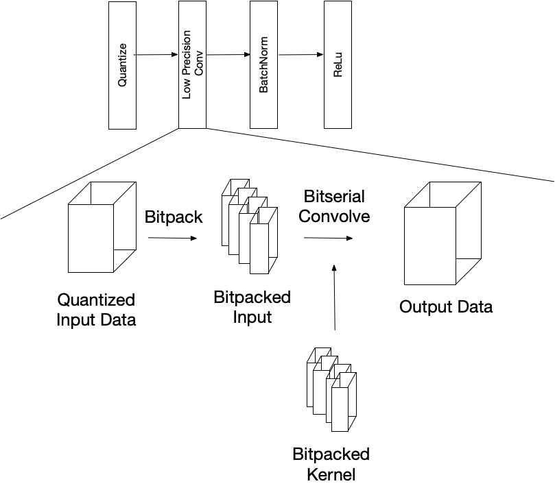
An example of a low precision graph snippet is below. The low precision convolution takes in quantized data and bitpacks into the proper data layout for an efficient bitserial convolution. The output is in a higher precision and traditional deep learning layers such as batch normalization and ReLu are applied to it, before being re-quantized and sent through another low precision operator.
Theoretically, low precision operators use less operations than floating point operators, leading many to believe they can achieve up tremendous speedups. However, deep learning frameworks leverage decades of engineering work through low level BLAS and LAPACK libraries that are incredibly well optimized, and CPUs include intrinsic instructions to accelerate these tasks. In practice, it is not simple to develop low-level operators such as convolutions that are competitive with 8-bit quantized or even floating point operators. In this post we introduce our approach to automatically generating optimized low precision convolutions for CPUs. We declare our low precision operators so that they compute on efficiently stored low precision inputs, and describe a schedule that describes a search space of implementation parameters. We rely on AutoTVM to quickly search the space and find optimized parameters for the particular convolution, precision, and backend.
Bitserial Computation Background
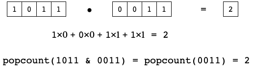
The core of low precision models is the bitserial dot product that enables convolution and dense operators to be computed using only bitwise operations and popcount. Typically, a dot product is computed by element wise multiplication of two vectors followed by summing all the elements, like the simple example below. If all the data is binary, the input vectors can be packed into single integer, and the dot product can be computed by bitwise-anding the packed inputs and counting the number of 1’s in the result using popcount. Note: Depending how the input data is quantized, bitwise-xnor may be used instead of bitwise-and.
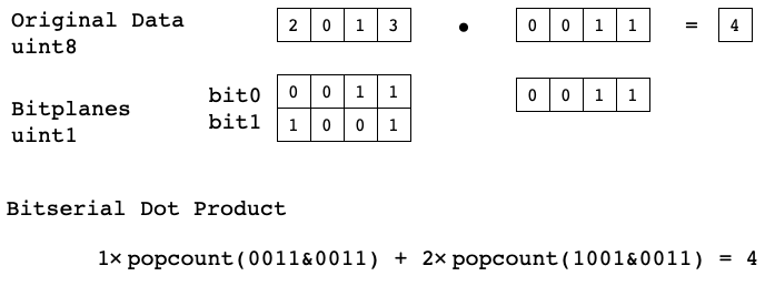
Arbitrary precision dot products can be computed in this fashion by first separating input data into bitplanes. Once in this representation we can compute dotproduct by summing weighted binary dot products between the bitplanes of A and B. The number of binary dotproducts grows with the product of A and B’s precision, so this method is only practical for very low precision data.
Defining Operators in TVM
Before the computation, input data needs to be bitpacked so that the bitplanes of the input data can be accessed and are packed into a supported datatype such as a uint8 or uint32. We provide a flexible bitpacking operator that takes arbitrary size input tensors and returns a bitpacked tensor where the user specifies which axis the bitplanes should be.
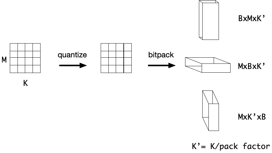
Once in this bitpacked format the low precision convolution can be computed bitserially. For this demo, that data is packed along the input channel and the bitplanes are added to the innermost axis, and the data is packed into 32-bit integers. The bitserial convolution is computed similar to a normal convolution, but the bitwise-and (&) replaces multiplication, and we use popcount to accumulate values in the packed data. The bitplane axes become additional reduction axes and compute the binary dot products between different bitplanes of the input and kernel. Finally, the output is computed in an unpacked format and in higher precision.
Input_bitpacked = bitpack(Input, activation_bits, pack_axis=3, bit_axis=4, pack_type=’uint32’)
Weights_bitpacked = bitpack(Filter, weight_bits, pack_axis=2, bit_axis=4, pack_type=’uint32’)
batch, in_height, in_width, in_channel_q, _ = Input_bitpacked.shape
kernel_h, kernel_w, _, num_filter, _ = Filter_bitpakced.shape

stride_h, stride_w = stride
pad_top, pad_left, pad_down, pad_right = get_pad_tuple(padding, (kernel_h, kernel_w))

# Computing the output shape
out_channel = num_filter
out_height = simplify((in_height - kernel_h + pad_top + pad_down) // stride_h + 1)
out_width = simplify((in_width - kernel_w + pad_left + pad_right) // stride_w + 1)
pad_before = [0, pad_top, pad_left, 0, 0]
pad_after = [0, pad_down, pad_right, 0, 0]
Input_padded = pad(Input_bitpacked, pad_before, pad_after, name="PaddedInput")

# Treat the bitplane axes like additional reduction axes
rc = tvm.reduce_axis((0, in_channel_q), name='rc')
ry = tvm.reduce_axis((0, kernel_h), name='ry')
rx = tvm.reduce_axis((0, kernel_w), name='rx')
ib = tvm.reduce_axis((0, input_bits), name='ib')
wb = tvm.reduce_axis((0, weight_bits), name='wb')


tvm.compute((batch, out_height, out_width, out_channel), lambda nn, yy, xx, ff:
             tvm.sum(tvm.popcount(
               Input_padded[nn, yy * stride_h + ry, xx * stride_w + rx, rc, ib] &
               Weights_bitpacked[ry, rx, rc, ff, wb])) << (ib+wb))).astype(out_dtype),
               axis=[rc, ry, rx, wb, ib]))
In our schedule we apply common optimizations like vectorization and memory tiling to provide better memory locality and take advantage of SIMD units. Some of these optimizations such as tiling, require parameters that need to be tuned to for the specific microarchitecture. We expose these parameters as knobs to TVM and use AutoTVM to automatically tune all the parameters simultaneously.
Finally, we can craft small microkernels to replace the innermost loop(s) of computation and schedule them using TVM’s tensorize primitive. Since, compilers often produce suboptimal code, people can often write short assembly sequences that are more efficient. These microkernels often take advantage of new intrinsics that are being introduced to help accelerate deep learning workloads and use them clever ways to improve memory accesses or reduce the number instructions required.
Results
Raspberry Pi
Convolution speedups on Raspberry Pi 3B compared to 16-bit integer TVM implementation. Workload are convolution layers from ResNet18.
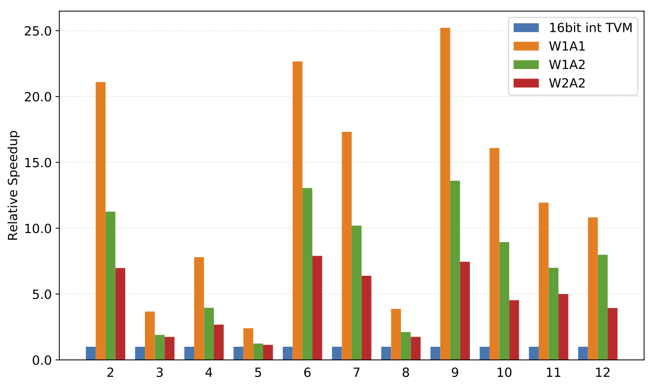
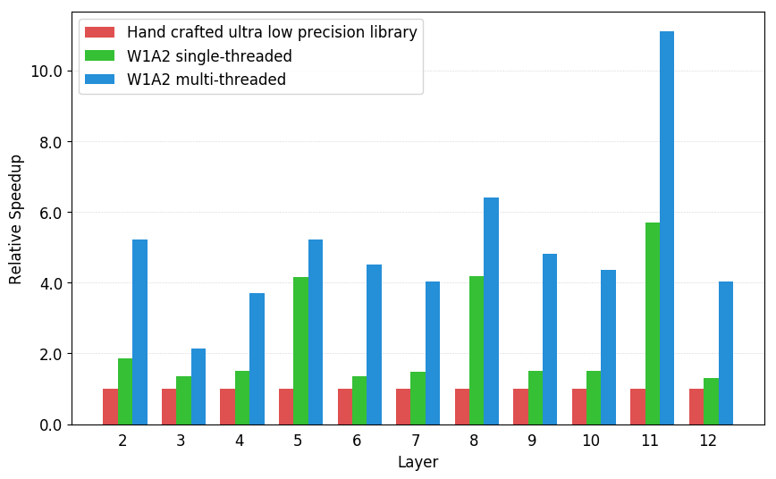
2-bit activation, 1-bit weight convolution speedups on Raspberry Pi 3B compared to hand optimized implementation from High performance ultra-low-precision convolutions on mobile devices.. Workload are convolution layers from ResNet18.
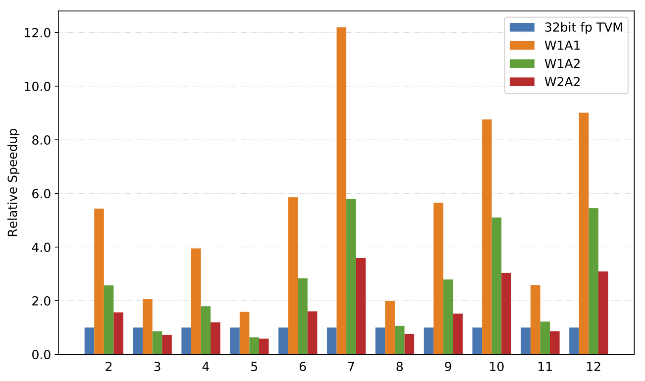
x86
Convolution speedups on x86 compared to a 32-bit floating point TVM implementation. Note: x86 doesn’t support a vectorized popcount for this microarchitecture, so speedups are lower.