Introduction to Relay IR
This article introduces Relay IR – the second generation of NNVM. We expect readers from two kinds of background – those who have a programming language background and deep learning framework developers who are familiar with the computational graph representation.
We briefly summarize the design goal here, and will touch upon these points in the later part of the article.
Support traditional data flow-style programming and transformations.
Support functional-style scoping, let-binding and making it a fully featured differentiable language.
Being able to allow the user to mix the two programming styles.
Build a Computational Graph with Relay
Traditional deep learning frameworks use computational graphs as their intermediate representation. A computational graph (or dataflow graph), is a directed acyclic graph (DAG) that represents the computation. Though dataflow graphs are limited in terms of the computations they are capable of expressing due to lacking control flow, their simplicity makes it easier to implement automatic differentiation and compile for heterogeneous execution environments (e.g., executing parts of the graph on specialized hardware).
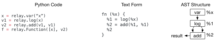
You can use Relay to build a computational (dataflow) graph. Specifically, the above code shows how to construct a simple two-node graph. You can find that the syntax of the example is not that different from existing computational graph IR like NNVMv1, with the only difference in terms of terminology:
Existing frameworks usually use graph and subgraph
Relay uses function e.g. –
fn (%x), to indicate the graph
Each dataflow node is a CallNode in Relay. The Relay Python DSL allows you to construct a dataflow graph quickly.
One thing we want to highlight in the above code – is that we explicitly constructed an Add node with
both input point to %1. When a deep learning framework evaluates the above program, it will compute
the nodes in topological order, and %1 will only be computed once.
While this fact is very natural to deep learning framework builders, it is something that might
surprise a PL researcher in the first place. If we implement a simple visitor to print out the result and
treat the result as nested Call expression, it becomes log(%x) + log(%x).
Such ambiguity is caused by different interpretations of program semantics when there is a shared node in the DAG.
In a normal functional programming IR, nested expressions are treated as expression trees, without considering the
fact that the %1 is actually reused twice in %2.
The Relay IR is mindful of this difference. Usually, deep learning framework users build the computational
graph in this fashion, where a DAG node reuse often occurs. As a result, when we print out the Relay program in
the text format, we print one CallNode per line and assign a temporary id (%1, %2) to each CallNode so each common
node can be referenced in later parts of the program.
Module: Support Multiple Functions (Graphs)
So far we have introduced how can we build a dataflow graph as a function. One might naturally ask: Can we support multiple functions and enable them to call each other? Relay allows grouping multiple functions together in a module; the code below shows an example of a function calling another function.
def @muladd(%x, %y, %z) {
  %1 = mul(%x, %y)
  %2 = add(%1, %z)
  %2
}
def @myfunc(%x) {
  %1 = @muladd(%x, 1, 2)
  %2 = @muladd(%1, 2, 3)
  %2
}
The Module can be viewed as a Map<GlobalVar, Function>. Here GlobalVar is just an id that is used to represent the functions
in the module. @muladd and @myfunc are GlobalVars in the above example. When a CallNode is used to call another function,
the corresponding GlobalVar is stored in the op field of the CallNode. It contains a level of indirection – we need to look up
body of the called function from the module using the corresponding GlobalVar. In this particular case, we could also directly
store the reference to the Function as op in the CallNode. So, why do we need to introduce GlobalVar? The main reason is that
GlobalVar decouples the definition/declaration and enables recursion and delayed declaration of the function.
def @myfunc(%x) {
  %1 = equal(%x, 1)
   if (%1) {
      %x
   } else {
     %2 = sub(%x, 1)
     %3 = @myfunc(%2)
      %4 = add(%3, %3)
      %4
  }
}
In the above example, @myfunc recursively calls itself. Using GlobalVar @myfunc to represent the function avoids
the cyclic dependency in the data structure.
At this point, we have introduced the basic concepts in Relay. Notably, Relay has the following improvements over NNVMv1:
Succinct text format that eases debugging of writing passes.
First-class support for subgraphs-functions, in a joint module, this enables further chance of joint optimizations such as inlining and calling convention specification.
Naive front-end language interop, for example, all the data structure can be visited in Python, which allows quick prototyping of optimizations in Python and mixing them with C++ code.
Let Binding and Scopes
So far, we have introduced how to build a computational graph in the good old way used in deep learning frameworks. This section will talk about a new important construct introduced by Relay – let bindings.
Let binding is used in every high-level programming language. In Relay, it is a data structure with three
fields Let(var, value, body). When we evaluate a let expression, we first evaluate the value part, assign
it to the var, then return the evaluated result in the body expression.
You can use a sequence of let bindings to construct a logically equivalent program to a dataflow program. The code example below shows one program with two forms side by side.
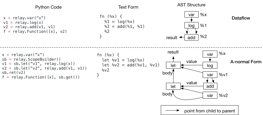
The nested let binding is called A-normal form, and it is commonly used as IRs in functional programming languages. Now, please take a close look at the AST structure. While the two programs are semantically identical (so are their textual representations, except that A-normal form has let prefix), their AST structures are different.
Since program optimizations take these AST data structures and transform them, the two different structures will
affect the compiler code we are going to write. For example, if we want to detect a pattern add(log(x), y):
In the data-flow form, we can first access the add node, then directly look at its first argument to see if it is a log
In the A-normal form, we cannot directly do the check anymore, because the first input to add is
%v1– we will need to keep a map from variable to its bound values and look up that map, in order to know that%v1is a log.
Different data structures will impact how you might write transformations, and we need to keep that in mind. So now, as a deep learning framework developer, you might ask, Why do we need let bindings? Your PL friends will always tell you that let is important – as PL is a quite established field, there must be some wisdom behind that.
Why We Might Need Let Binding
One key usage of let binding is that it specifies the scope of computation. Let us take a look at the following example, which does not use let bindings.
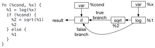
The problem comes when we try to decide where we should evaluate node %1. In particular, while the text format seems
to suggest that we should evaluate node %1 outside the if scope, the AST(as shown in the picture) does not suggest so.
Actually, a dataflow graph never defines its scope of the evaluation. This introduces some ambiguity in the semantics.
This ambiguity becomes more interesting when we have closures. Consider the following program, which returns a closure.
We don’t know where should we compute %1; it can be either inside or outside the closure.
fn (%x) {
  %1 = log(%x)
  %2 = fn(%y) {
    add(%y, %1)
  }
  %2
}
A let binding solves this problem, as the computation of the value happens at the let node. In both programs,
if we change %1 = log(%x) to let %v1 = log(%x), we clearly specify the computation location to
be outside of the if scope and closure. As you can see let-binding gives a more precise specification of the computation site
and could be useful when we generate backend code (as such specification is in the IR).
On the other hand, the dataflow form, which does not specify the scope of computation, does have its own advantages – namely, we don’t need to worry about where to put the let when we generate the code. The dataflow form also gives more freedom to the later passes to decide where to put the evaluation point. As a result, it might not be a bad idea to use data flow form of the program in the initial phases of optimizations when you find it is convenient. Many optimizations in Relay today are written to optimize dataflow programs.
However, when we lower the IR to an actual runtime program, we need to be precise about the scope of computation. In particular, we want to explicitly specify where the scope of computation should happen when we are using sub-functions and closures. Let-binding can be used to solve this problem in later stage execution specific optimizations.
Implication on IR Transformations
Hopefully, by now you are familiar with the two kinds of representations. Most functional programming languages do their analysis in A-normal form, where the analyzer does not need to be mindful that the expressions are DAGs.
Relay choose to support both the dataflow form and let bindings. We believe that it is important to let the framework developer choose the representation they are familiar with. This does, however, have some implications on how we write passes:
If you come from a dataflow background and want to handle lets, keep a map of var to the expressions so you can perform lookup when encountering a var. This likely means a minimum change as we already need a map from expressions to transformed expressions anyway. Note that this will effectively remove all the lets in the program.
If you come from a PL background and like A-normal form, we will provide a dataflow to A-normal form pass.
For PL folks, when you are implementing something (like a dataflow-to-ANF transformation), be mindful that expressions can be DAGs, and this usually means that we should visit expressions with a
Map<Expr, Result>and only compute the transformed result once, so the resulting expression keeps the common structure.
There are additional advanced concepts such as symbolic shape inference, polymorphic functions that are not covered by this material; you are more than welcome to look at other materials.