
Note
Click here to download the full example code
Simple Matrix Multiply
Author: Thierry Moreau
In this tutorial, we will build on top of the Get Started with VTA tutorial and introduce additional concepts required to implement matrix multiplication on VTA with the TVM workflow.
RPC Setup
We start by programming the Pynq’s FPGA and building its RPC runtime as we did in the VTA introductory tutorial.
from __future__ import absolute_import, print_function

import os
import tvm
from tvm import te
import vta
import numpy as np
from tvm import rpc
from tvm.contrib import utils
from vta.testing import simulator

# Load VTA parameters from the 3rdparty/vta-hw/config/vta_config.json file
env = vta.get_env()

# We read the Pynq RPC host IP address and port number from the OS environment
host = os.environ.get("VTA_RPC_HOST", "192.168.2.99")
port = int(os.environ.get("VTA_RPC_PORT", "9091"))

# We configure both the bitstream and the runtime system on the Pynq
# to match the VTA configuration specified by the vta_config.json file.
if env.TARGET == "pynq" or env.TARGET == "de10nano":

    # Make sure that TVM was compiled with RPC=1
    assert tvm.runtime.enabled("rpc")
    remote = rpc.connect(host, port)

    # Reconfigure the JIT runtime
    vta.reconfig_runtime(remote)

    # Program the FPGA with a pre-compiled VTA bitstream.
    # You can program the FPGA with your own custom bitstream
    # by passing the path to the bitstream file instead of None.
    vta.program_fpga(remote, bitstream=None)

# In simulation mode, host the RPC server locally.
elif env.TARGET in ["sim", "tsim"]:
    remote = rpc.LocalSession()
Computation Declaration
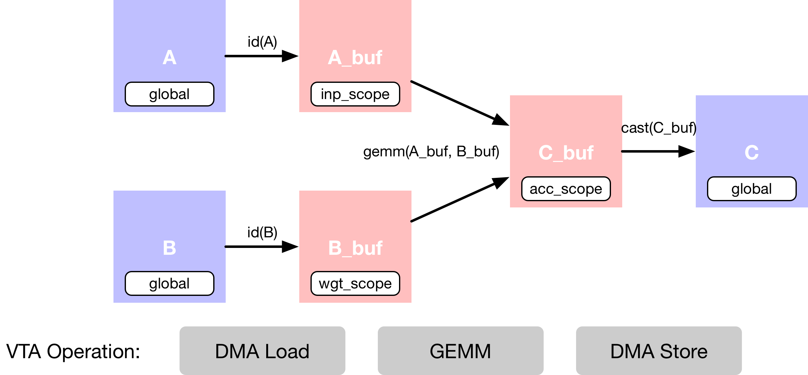
In this example we describe a simple matrix multiplication addition, which
requires multiple computation stages, as shown in the dataflow diagram below.
First we describe the input tensors A and B that are living
in main memory.
Second, we need to declare intermediate tensors A_buf and
B_buf, which will live in VTA’s on-chip buffers.
Having this extra computational stage allows us to explicitly
stage cached reads and writes.
Third, we describe the matrix multiplication computation over
A_buf and B_buf to produce the product matrix C_buf.
The last operation is a cast and copy back to DRAM, into results tensor
C.
Data Layout
We describe the placeholder tensors A, and B in a tiled data
format to match the data layout requirements imposed by the VTA tensor core.
Note
Data Tiling
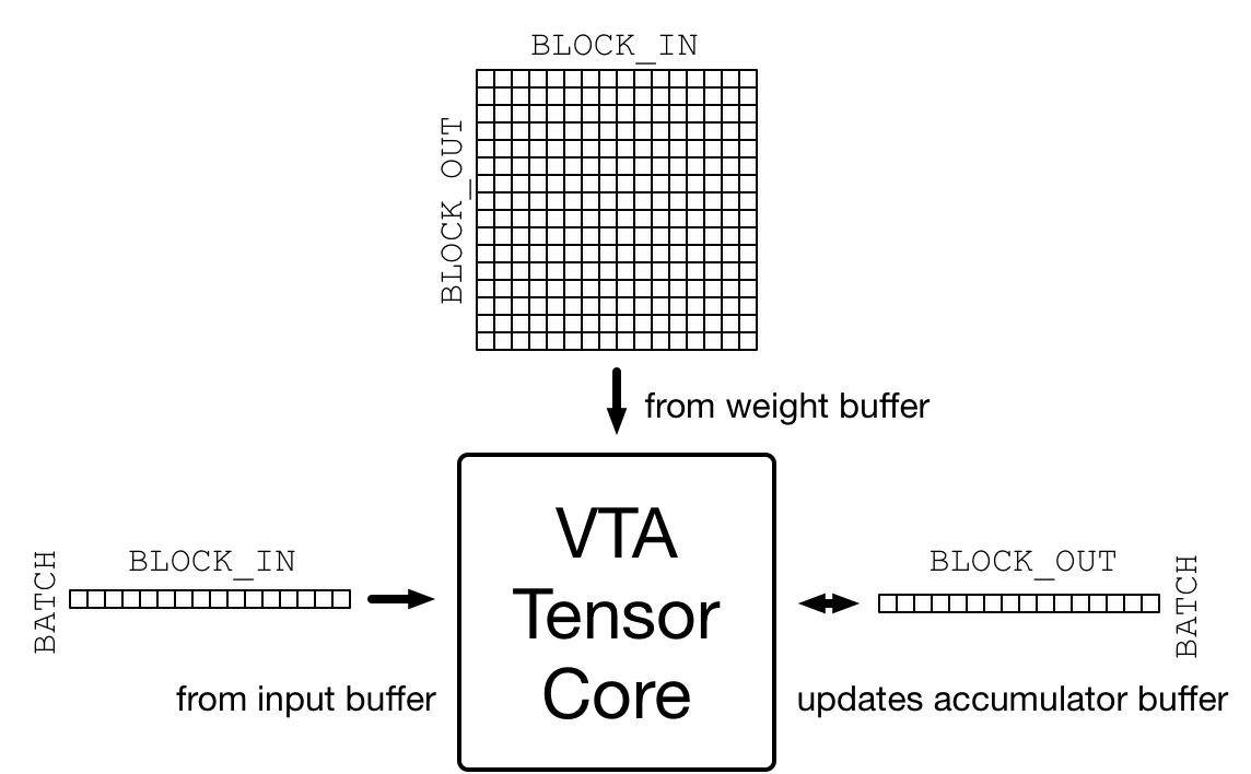
One source of complexity when targeting accelerators is to make sure that the data layout matches the layout imposed by the accelerator design. VTA is designed around a tensor core that performs, one matrix-matrix operation per cycle between an activation matrix and a weight matrix, adding the result matrix to an accumulator matrix, as shown in the figure below.
The dimensions of that matrix-matrix multiplication are specified in
the vta_config.json configuration file.
The activation matrix has a (BATCH, BLOCK_IN) shape
and the transposed weight matrix has a (BLOCK_OUT, BLOCK_IN) shape,
thus inferring that the resulting output matrix has a
(BATCH, BLOCK_OUT) shape.
Consequently input and output tensors processed by VTA need to be
tiled according to these aforementioned dimension.
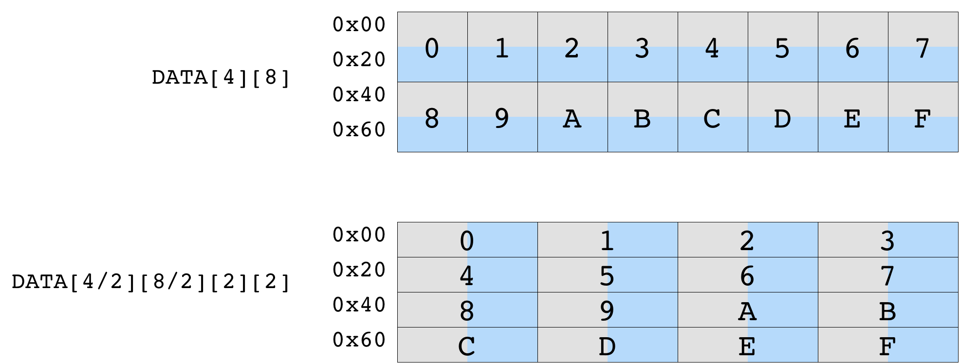
The diagram below shows the impact of data tiling on a matrix that is originally of shape (4, 8). Tiling by a (2, 2) tile shape ensures that data within each tile is contiguous. The resulting tiled tensor has a shape of (2, 4, 2, 2).
We first define the variables m, n, o to represent
the shape of the matrix multiplication. These variables are multiplicative
factors over the BLOCK_OUT, BLOCK_IN, and BATCH
tensor dimensions respectively.
By default, the configuration file sets BATCH, BLOCK_IN, and
BLOCK_OUT to be 1, 16 and 16 respectively (BATCH being set to
1 implies that our compute building block is vector-matrix multiply).
Note
Data Types
It’s important to not only match the inner-tile
dimension of VTA’s tensor core, but also to match the specific data types
expected by VTA.
VTA for now only supports fixed point data types, which integer width is
specified in the vta_config.json file by INP_WIDTH and
WGT_WIDTH for the activations and weights data types respectively.
In addition, the accumulator data type integer width is specified by
ACC_WIDTH.
By default, the configuration file sets INP_WIDTH
and WGT_WIDTH to 8.
The accumulator width ACC_WIDTH is set to 32, in order to avoid
overflow during accumulation.
As a result, env.inp_dtype and env.wgt_dtype are all
narrow 8-bit integers, while env.acc_dtype is a standard 32-bit
integer.
# Output channel factor m - total 16x16=256 output channels
m = 16
# Input channel factor n - total 16x16=256 input channels
n = 16
# Batch factor o (we use single batch inference)
o = 1
# A placeholder tensor in tiled data format
A = te.placeholder((o, n, env.BATCH, env.BLOCK_IN), name="A", dtype=env.inp_dtype)
# B placeholder tensor in tiled data format
B = te.placeholder((m, n, env.BLOCK_OUT, env.BLOCK_IN), name="B", dtype=env.wgt_dtype)
# A copy buffer
A_buf = te.compute((o, n, env.BATCH, env.BLOCK_IN), lambda *i: A(*i), "A_buf")
# B copy buffer
B_buf = te.compute((m, n, env.BLOCK_OUT, env.BLOCK_IN), lambda *i: B(*i), "B_buf")
Matrix Multiplication
Now we’re ready to describe the matrix multiplication result tensor C,
with another compute operation.
The compute function takes the shape of the tensor, as well as a lambda
function that describes the computation rule for each position of the tensor.
In order to implement matrix multiplication, the lambda function needs to
include a reduction formula over the input channel dimension axes.
To create a reduction formula, we can declare a reduction axis using
te.reduce_axis, which takes in the range of reductions.
te.sum takes in the expression to be reduced as well as
the reduction axes to compute the sum of value over all k in the declared
ranges.
Note that the reduction needs to be performed over 32-bit env.acc_dtype
accumulator data types.
No computation happens during this phase, as we are only declaring how the computation should be done.
# Outer input feature reduction axis
ko = te.reduce_axis((0, n), name="ko")
# Inner input feature reduction axis
ki = te.reduce_axis((0, env.BLOCK_IN), name="ki")
# Describe the in-VTA matrix multiplication
C_buf = te.compute(
    (o, m, env.BATCH, env.BLOCK_OUT),
    lambda bo, co, bi, ci: te.sum(
        A_buf[bo, ko, bi, ki].astype(env.acc_dtype) * B_buf[co, ko, ci, ki].astype(env.acc_dtype),
        axis=[ko, ki],
    ),
    name="C_buf",
)
Casting the Results
After the computation is done, we’ll need to send the results computed by VTA back to main memory.
Note
Memory Store Restrictions
One specificity of VTA is that it only supports DRAM stores in the narrow
env.inp_dtype data type format.
This lets us reduce the data footprint for memory transfers, but also lets
us quantize the wide accumulator data type down to a data format that
matches the input activation data type.
This means that in the context of neural network inference, the outputs
of a given layer after activation can be consumed directly by the next
layer.
We perform one last typecast operation to the narrow input activation data format.
# Cast to output type, and send to main memory
C = te.compute(
    (o, m, env.BATCH, env.BLOCK_OUT), lambda *i: C_buf(*i).astype(env.inp_dtype), name="C"
)
This concludes the computation declaration part of this tutorial.
Scheduling the Computation
While the above lines describes the computation rule, we can obtain
C in many ways.
TVM asks the user to provide an implementation of the computation called
schedule.
A schedule is a set of transformations to an original computation that transforms the implementation of the computation without affecting correctness. This simple VTA programming tutorial aims to demonstrate basic schedule transformations that will map the original schedule down to VTA hardware primitives.
Default Schedule
After we construct the schedule, by default the schedule computes
C in the following way:
# Let's take a look at the generated schedule
s = te.create_schedule(C.op)
print(tvm.lower(s, [A, B, C], simple_mode=True))
Out:
primfn(A_1: handle, B_1: handle, C_1: handle) -> ()
  attr = {"from_legacy_te_schedule": True, "global_symbol": "main", "tir.noalias": True}
  buffers = {C: Buffer(C_2: Pointer(int8), int8, [1, 16, 1, 16], []),
             A: Buffer(A_2: Pointer(int8), int8, [1, 16, 1, 16], []),
             B: Buffer(B_2: Pointer(int8), int8, [16, 16, 16, 16], [])}
  buffer_map = {A_1: A, B_1: B, C_1: C} {
  allocate(A_buf: Pointer(global int8), int8, [256]), storage_scope = global;
  allocate(B_buf: Pointer(global int8), int8, [65536]), storage_scope = global;
  allocate(C_buf: Pointer(global int32), int32, [256]), storage_scope = global {
    for (i1: int32, 0, 16) {
      for (i3: int32, 0, 16) {
        A_buf[((i1*16) + i3)] = (int8*)A_2[((i1*16) + i3)]
      }
    }
    for (i0: int32, 0, 16) {
      for (i1_1: int32, 0, 16) {
        for (i2: int32, 0, 16) {
          for (i3_1: int32, 0, 16) {
            B_buf[((((i0*4096) + (i1_1*256)) + (i2*16)) + i3_1)] = (int8*)B_2[((((i0*4096) + (i1_1*256)) + (i2*16)) + i3_1)]
          }
        }
      }
    }
    for (co: int32, 0, 16) {
      for (ci: int32, 0, 16) {
        C_buf[((co*16) + ci)] = 0
        for (ko: int32, 0, 16) {
          for (ki: int32, 0, 16) {
            C_buf[((co*16) + ci)] = ((int32*)C_buf[((co*16) + ci)] + (cast(int32, (int8*)A_buf[((ko*16) + ki)])*cast(int32, (int8*)B_buf[((((co*4096) + (ko*256)) + (ci*16)) + ki)])))
          }
        }
      }
    }
    for (i1_2: int32, 0, 16) {
      for (i3_2: int32, 0, 16) {
        C_2[((i1_2*16) + i3_2)] = cast(int8, (int32*)C_buf[((i1_2*16) + i3_2)])
      }
    }
  }
}
Although this schedule makes sense, it won’t compile to VTA. In order to obtain correct code generation, we need to apply scheduling primitives and code annotation that will transform the schedule into one that can be directly lowered onto VTA hardware intrinsics. Those include:
DMA copy operations which will take globally-scoped tensors and copy those into locally-scoped tensors.
Tensor operations that will perform the matrix multiplication.
Buffer Scopes
First, we set the scope of the buffers to tell TVM that these buffers
will be living in the VTA’s on-chip SRAM caches.
Below, we tell TVM that A_buf, B_buf, C_buf
will respectively live in VTA’s on-chip input, weight and accumulator
memory.
Note
VTA’s On-Chip SRAMs
VTA has three different memory scopes, each corresponding to different on-chip SRAM buffers.
env.inp_scope: Input buffer, which is a read-only SRAM buffer that stores input matrices of shape(env.BATCH, env.BLOCK_IN)of typeenv.inp_dtype. The input buffer contains 2 ^ LOG_INP_BUFF_SIZE matrix elements (as specified in thevta_config.jsonfile).
env.wgt_scope: Weight buffer, which is a read-only SRAM buffer that stores weight matrices of shape(env.BLOCK_OUT, env.BLOCK_IN)of typeenv.wgt_dtype. The weight buffer contains 2 ^ LOG_WGT_BUFF_SIZE matrix elements.
env.acc_scope: Accumulator buffer, which is a read/write SRAM buffer that stores accumulator matrices of shape(env.BATCH, env.BLOCK_OUT)of typeenv.acc_dtype. The accumulator buffer is VTA’s general purpose register file: it holds both intermediate results of convolutions and matrix multiplications as well as intermediate results of pooling, batch normalization, and activation layers. The accumulator buffer contains 2 ^ LOG_ACC_BUFF_SIZE matrix elements.
# Set the intermediate tensor's scope to VTA's on-chip buffers
s[A_buf].set_scope(env.inp_scope)
s[B_buf].set_scope(env.wgt_scope)
s[C_buf].set_scope(env.acc_scope)
DMA Transfers
We need to schedule DMA transfers to move data living in DRAM to
and from the VTA on-chip buffers.
This can be achieved using the compute_at schedule primitive
which nests the copying of the buffers into the computation loop
that performs the matrix multiplication.
We insert dma_copy pragmas to indicate to the compiler
that the copy operations will be performed in bulk via DMA,
which is common in hardware accelerators.
Finally, we print the temporary schedule to observe the effects of
moving the copy operations into the matrix multiplication loop.
# Move buffer copy into matrix multiply loop
s[A_buf].compute_at(s[C_buf], ko)
s[B_buf].compute_at(s[C_buf], ko)

# Tag the buffer copies with the DMA pragma to insert a DMA transfer
s[A_buf].pragma(s[A_buf].op.axis[0], env.dma_copy)
s[B_buf].pragma(s[B_buf].op.axis[0], env.dma_copy)
s[C].pragma(s[C].op.axis[0], env.dma_copy)

# Let's take a look at the transformed schedule
print(tvm.lower(s, [A, B, C], simple_mode=True))
Out:
primfn(A_1: handle, B_1: handle, C_1: handle) -> ()
  attr = {"from_legacy_te_schedule": True, "global_symbol": "main", "tir.noalias": True}
  buffers = {C: Buffer(C_2: Pointer(int8), int8, [1, 16, 1, 16], []),
             A: Buffer(A_2: Pointer(int8), int8, [1, 16, 1, 16], []),
             B: Buffer(B_2: Pointer(int8), int8, [16, 16, 16, 16], [])}
  buffer_map = {A_1: A, B_1: B, C_1: C} {
  allocate(C_buf: Pointer(local.acc_buffer int32), int32, [256]), storage_scope = local.acc_buffer;
  allocate(A_buf: Pointer(local.inp_buffer int8), int8, [16]), storage_scope = local.inp_buffer;
  allocate(B_buf: Pointer(local.wgt_buffer int8), int8, [16]), storage_scope = local.wgt_buffer {
    for (co: int32, 0, 16) {
      for (ci: int32, 0, 16) {
        C_buf[((co*16) + ci)] = 0
        for (ko: int32, 0, 16) {
          attr [IterVar(i0: int32, (nullptr), "DataPar", "")] "pragma_dma_copy" = 1;
          for (i3: int32, 0, 16) {
            A_buf[i3] = (int8*)A_2[((ko*16) + i3)]
          }
          attr [IterVar(i0_1: int32, (nullptr), "DataPar", "")] "pragma_dma_copy" = 1;
          for (i3_1: int32, 0, 16) {
            B_buf[i3_1] = (int8*)B_2[((((co*4096) + (ko*256)) + (ci*16)) + i3_1)]
          }
          for (ki: int32, 0, 16) {
            C_buf[((co*16) + ci)] = ((int32*)C_buf[((co*16) + ci)] + (cast(int32, (int8*)A_buf[ki])*cast(int32, (int8*)B_buf[ki])))
          }
        }
      }
    }
    attr [IterVar(i0_2: int32, (nullptr), "DataPar", "")] "pragma_dma_copy" = 1;
    for (i1: int32, 0, 16) {
      for (i3_2: int32, 0, 16) {
        C_2[((i1*16) + i3_2)] = cast(int8, (int32*)C_buf[((i1*16) + i3_2)])
      }
    }
  }
}
Tensorization
The last step of the schedule transformation consists in applying tensorization to our schedule. Tensorization is analogous to vectorization, but extends the concept to a higher-dimensional unit of computation. Consequently, tensorization imposes data layout constraints as discussed earlier when declaring the data layout input placeholders. We’ve already arranged our tensors in a tiled format, so the next thing we need to perform is loop reordering to accommodate for tensorization.
Here we choose to move the outermost reduction axis all the way out.
This dictates that we first iterate over input channels, then batch
dimensions, and finally output channels.
Lastly, we apply the tensorization scheduling primitive tensorize
along the outer axis of the inner-most matrix matrix multiplication tensor
block.
We print the finalized schedule that is ready for code-generation
by the VTA runtime JIT compiler.
s[C_buf].reorder(
    ko, s[C_buf].op.axis[0], s[C_buf].op.axis[1], s[C_buf].op.axis[2], s[C_buf].op.axis[3], ki
)
s[C_buf].tensorize(s[C_buf].op.axis[2], env.gemm)

# Let's take a look at the finalized schedule
print(vta.lower(s, [A, B, C], simple_mode=True))
Out:
primfn(A_1: handle, B_1: handle, C_1: handle) -> ()
  attr = {"from_legacy_te_schedule": True, "global_symbol": "main", "tir.noalias": True}
  buffers = {C: Buffer(C_2: Pointer(int8), int8, [1, 16, 1, 16], []),
             A: Buffer(A_2: Pointer(int8), int8, [1, 16, 1, 16], []),
             B: Buffer(B_2: Pointer(int8), int8, [16, 16, 16, 16], [])}
  buffer_map = {A_1: A, B_1: B, C_1: C} {
  attr [IterVar(vta: int32, (nullptr), "ThreadIndex", "vta")] "coproc_scope" = 2 {
    attr [IterVar(vta, (nullptr), "ThreadIndex", "vta")] "coproc_uop_scope" = "VTAPushGEMMOp" {
      @tir.call_extern("VTAUopLoopBegin", 16, 1, 0, 0, dtype=int32)
      @tir.vta.uop_push(0, 1, 0, 0, 0, 0, 0, 0, dtype=int32)
      @tir.call_extern("VTAUopLoopEnd", dtype=int32)
    }
    @tir.vta.coproc_dep_push(2, 1, dtype=int32)
  }
  for (ko: int32, 0, 16) {
    attr [IterVar(vta, (nullptr), "ThreadIndex", "vta")] "coproc_scope" = 1 {
      @tir.vta.coproc_dep_pop(2, 1, dtype=int32)
      @tir.call_extern("VTALoadBuffer2D", @tir.tvm_thread_context(@tir.vta.command_handle(, dtype=handle), dtype=handle), A_2, ko, 1, 1, 1, 0, 0, 0, 0, 0, 2, dtype=int32)
      @tir.call_extern("VTALoadBuffer2D", @tir.tvm_thread_context(@tir.vta.command_handle(, dtype=handle), dtype=handle), B_2, ko, 1, 16, 16, 0, 0, 0, 0, 0, 1, dtype=int32)
      @tir.vta.coproc_dep_push(1, 2, dtype=int32)
    }
    attr [IterVar(vta, (nullptr), "ThreadIndex", "vta")] "coproc_scope" = 2 {
      @tir.vta.coproc_dep_pop(1, 2, dtype=int32)
      attr [IterVar(vta, (nullptr), "ThreadIndex", "vta")] "coproc_uop_scope" = "VTAPushGEMMOp" {
        @tir.call_extern("VTAUopLoopBegin", 16, 1, 0, 1, dtype=int32)
        @tir.vta.uop_push(0, 0, 0, 0, 0, 0, 0, 0, dtype=int32)
        @tir.call_extern("VTAUopLoopEnd", dtype=int32)
      }
      @tir.vta.coproc_dep_push(2, 1, dtype=int32)
    }
  }
  @tir.vta.coproc_dep_push(2, 3, dtype=int32)
  @tir.vta.coproc_dep_pop(2, 1, dtype=int32)
  attr [IterVar(vta, (nullptr), "ThreadIndex", "vta")] "coproc_scope" = 3 {
    @tir.vta.coproc_dep_pop(2, 3, dtype=int32)
    @tir.call_extern("VTAStoreBuffer2D", @tir.tvm_thread_context(@tir.vta.command_handle(, dtype=handle), dtype=handle), 0, 4, C_2, 0, 16, 1, 16, dtype=int32)
  }
  @tir.vta.coproc_sync(, dtype=int32)
}
This concludes the scheduling portion of this tutorial.
TVM Compilation
After we have finished specifying the schedule, we can compile it into a TVM function.
# Build GEMM VTA kernel
my_gemm = vta.build(s, [A, B, C], "ext_dev", env.target_host, name="my_gemm")

# Write the compiled module into an object file.
temp = utils.tempdir()
my_gemm.save(temp.relpath("gemm.o"))

# Send the executable over RPC
remote.upload(temp.relpath("gemm.o"))

# Load the compiled module
f = remote.load_module("gemm.o")
Running the Function
The compiled TVM function uses a concise C API and can be invoked from code language.
TVM provides an array API in python to aid quick testing and prototyping. The array API is based on DLPack standard.
We first create a remote context (for remote execution on the Pynq).
Then
tvm.nd.arrayformats the data accordingly.f()runs the actual computation.numpy()copies the result array back in a format that can be interpreted.
# Get the remote device context
ctx = remote.ext_dev(0)

# Initialize the A and B arrays randomly in the int range of (-128, 128]
A_orig = np.random.randint(-128, 128, size=(o * env.BATCH, n * env.BLOCK_IN)).astype(A.dtype)
B_orig = np.random.randint(-128, 128, size=(m * env.BLOCK_OUT, n * env.BLOCK_IN)).astype(B.dtype)

# Apply packing to the A and B arrays from a 2D to a 4D packed layout
A_packed = A_orig.reshape(o, env.BATCH, n, env.BLOCK_IN).transpose((0, 2, 1, 3))
B_packed = B_orig.reshape(m, env.BLOCK_OUT, n, env.BLOCK_IN).transpose((0, 2, 1, 3))

# Format the input/output arrays with tvm.nd.array to the DLPack standard
A_nd = tvm.nd.array(A_packed, ctx)
B_nd = tvm.nd.array(B_packed, ctx)
C_nd = tvm.nd.array(np.zeros((o, m, env.BATCH, env.BLOCK_OUT)).astype(C.dtype), ctx)

# Clear stats
if env.TARGET in ["sim", "tsim"]:
    simulator.clear_stats()

# Invoke the module to perform the computation
f(A_nd, B_nd, C_nd)
Verifying Correctness
Compute the reference result with numpy and assert that the output of the matrix multiplication indeed is correct
# Compute reference result with numpy
C_ref = np.dot(A_orig.astype(env.acc_dtype), B_orig.T.astype(env.acc_dtype)).astype(C.dtype)
C_ref = C_ref.reshape(o, env.BATCH, m, env.BLOCK_OUT).transpose((0, 2, 1, 3))
np.testing.assert_equal(C_ref, C_nd.numpy())

# Print stats
if env.TARGET in ["sim", "tsim"]:
    sim_stats = simulator.stats()
    print("Execution statistics:")
    for k, v in sim_stats.items():
        print("\t{:<16}: {:>16}".format(k, v))

print("Successful matrix multiply test!")
Out:
Execution statistics:
        inp_load_nbytes :              256
        wgt_load_nbytes :            65536
        acc_load_nbytes :                0
        uop_load_nbytes :                8
        out_store_nbytes:              256
        gemm_counter    :              256
        alu_counter     :                0
Successful matrix multiply test!
Summary
This tutorial showcases the TVM workflow to implement a simple matrix multiplication example on VTA. The general workflow includes:
Programming the FPGA with the VTA bitstream over RPC.
Describing matrix multiplication via a series of computations.
Describing how we want to perform the computation using schedule primitives.
Compiling the function to the VTA target.
Running the compiled module and verifying it against a numpy implementation.