5. Training Vision Models for microTVM on Arduino

Author: Gavin Uberti

This tutorial shows how MobileNetV1 models can be trained to fit on embedded devices, and how those models can be deployed to Arduino using TVM.

Motivation

When building IOT devices, we often want them to see and understand the world around them. This can take many forms, but often times a device will want to know if a certain kind of object is in its field of vision.

For example, a security camera might look for people, so it can decide whether to save a video to memory. A traffic light might look for cars, so it can judge which lights should change first. Or a forest camera might look for a kind of animal, so they can estimate how large the animal population is.

To make these devices affordable, we would like them to need only a low-cost processor like the nRF52840 (costing five dollars each on Mouser) or the RP2040 (just $1.45 each!).

These devices have very little memory (~250 KB RAM), meaning that no conventional edge AI vision model (like MobileNet or EfficientNet) will be able to run. In this tutorial, we will show how these models can be modified to work around this requirement. Then, we will use TVM to compile and deploy it for an Arduino that uses one of these processors.

Installing the Prerequisites

This tutorial will use TensorFlow to train the model - a widely used machine learning library created by Google. TensorFlow is a very low-level library, however, so we will the Keras interface to talk to TensorFlow. We will also use TensorFlow Lite to perform quantization on our model, as TensorFlow by itself does not support this.

Once we have our generated model, we will use TVM to compile and test it. To avoid having to build from source, we’ll install tlcpack - a community build of TVM. Lastly, we’ll also install imagemagick and curl to preprocess data:

pip install -q tensorflow tflite
pip install -q tlcpack-nightly -f https://tlcpack.ai/wheels
apt-get -qq install imagemagick curl

# Install Arduino CLI and library for Nano 33 BLE
curl -fsSL https://raw.githubusercontent.com/arduino/arduino-cli/master/install.sh | sh
/content/bin/arduino-cli core update-index
/content/bin/arduino-cli core install arduino:mbed_nano

Using the GPU

This tutorial demonstrates training a neural network, which is requires a lot of computing power and will go much faster if you have a GPU. If you are viewing this tutorial on Google Colab, you can enable a GPU by going to Runtime->Change runtime type and selecting “GPU” as our hardware accelerator. If you are running locally, you can follow TensorFlow’s guide instead.

We can test our GPU installation with the following code:

import tensorflow as tf

if not tf.test.gpu_device_name():
    print("No GPU was detected!")
    print("Model training will take much longer (~30 minutes instead of ~5)")
else:
    print("GPU detected - you're good to go.")

GPU detected - you're good to go.

Choosing Our Work Dir

We need to pick a directory where our image datasets, trained model, and eventual Arduino sketch will all live. If running on Google Colab, we’ll save everything in /root (aka ~) but you’ll probably want to store it elsewhere if running locally. Note that this variable only affects Python scripts - you’ll have to adjust the Bash commands too.

import os

FOLDER = "/root"

Downloading the Data

Convolutional neural networks usually learn by looking at many images, along with labels telling the network what those images are. To get these images, we’ll need a publicly available dataset with thousands of images of all sorts of objects and labels of what’s in each image. We’ll also need a bunch of images that aren’t of cars, as we’re trying to distinguish these two classes.

In this tutorial, we’ll create a model to detect if an image contains a car, but you can use whatever category you like! Just change the source URL below to one containing images of another type of object.

To get our car images, we’ll be downloading the Stanford Cars dataset, which contains 16,185 full color images of cars. We’ll also need images of random things that aren’t cars, so we’ll use the COCO 2017 validation set (it’s smaller, and thus faster to download than the full training set. Training on the full data set would yield better results). Note that there are some cars in the COCO 2017 data set, but it’s a small enough fraction not to matter - just keep in mind that this will drive down our percieved accuracy slightly.

We could use the TensorFlow dataloader utilities, but we’ll instead do it manually to make sure it’s easy to change the datasets being used. We’ll end up with the following file hierarchy:

/root
├── images
│   ├── object
│   │   ├── 000001.jpg
│   │   │ ...
│   │   └── 016185.jpg
│   ├── object.tgz
│   ├── random
│   │   ├── 000000000139.jpg
│   │   │ ...
│   │   └── 000000581781.jpg
│   └── random.zip

We should also note that Stanford cars has 8k images, while the COCO 2017 validation set is 5k images - it is not a 50/50 split! If we wanted to, we could weight these classes differently during training to correct for this, but training will still work if we ignore it. It should take about 2 minutes to download the Stanford Cars, while COCO 2017 validation will take 1 minute.

import os
import shutil
import urllib.request

# Download datasets
os.makedirs(f"{FOLDER}/downloads")
os.makedirs(f"{FOLDER}/images")
urllib.request.urlretrieve(
    "https://data.deepai.org/stanfordcars.zip", f"{FOLDER}/downloads/target.zip"
)
urllib.request.urlretrieve(
    "http://images.cocodataset.org/zips/val2017.zip", f"{FOLDER}/downloads/random.zip"
)

# Extract them and rename their folders
shutil.unpack_archive(f"{FOLDER}/downloads/target.zip", f"{FOLDER}/downloads")
shutil.unpack_archive(f"{FOLDER}/downloads/random.zip", f"{FOLDER}/downloads")
shutil.move(f"{FOLDER}/downloads/cars_train/cars_train", f"{FOLDER}/images/target")
shutil.move(f"{FOLDER}/downloads/val2017", f"{FOLDER}/images/random")

'/tmp/tmp0hsnny6a/images/random'

Loading the Data

Currently, our data is stored on-disk as JPG files of various sizes. To train with it, we’ll have to load the images into memory, resize them to be 64x64, and convert them to raw, uncompressed data. Keras’s image_dataset_from_directory will take care of most of this, though it loads images such that each pixel value is a float from 0 to 255.

We’ll also need to load labels, though Keras will help with this. From our subdirectory structure, it knows the images in /objects are one class, and those in /random another. Setting label_mode='categorical' tells Keras to convert these into categorical labels - a 2x1 vector that’s either [1, 0] for an object of our target class, or [0, 1] vector for anything else. We’ll also set shuffle=True to randomize the order of our examples.

We will also batch the data - grouping samples into clumps to make our training go faster. Setting batch_size = 32 is a decent number.

Lastly, in machine learning we generally want our inputs to be small numbers. We’ll thus use a Rescaling layer to change our images such that each pixel is a float between 0.0 and 1.0, instead of 0 to 255. We need to be careful not to rescale our categorical labels though, so we’ll use a lambda function.

IMAGE_SIZE = (64, 64, 3)
unscaled_dataset = tf.keras.utils.image_dataset_from_directory(
    f"{FOLDER}/images",
    batch_size=32,
    shuffle=True,
    label_mode="categorical",
    image_size=IMAGE_SIZE[0:2],
)
rescale = tf.keras.layers.Rescaling(scale=1.0 / 255)
full_dataset = unscaled_dataset.map(lambda im, lbl: (rescale(im), lbl))

Found 13144 files belonging to 2 classes.

What’s Inside Our Dataset?

Before giving this data set to our neural network, we ought to give it a quick visual inspection. Does the data look properly transformed? Do the labels seem appropriate? And what’s our ratio of objects to other stuff? We can display some examples from our datasets using matplotlib:

import matplotlib.pyplot as plt

num_target_class = len(os.listdir(f"{FOLDER}/images/target/"))
num_random_class = len(os.listdir(f"{FOLDER}/images/random/"))
print(f"{FOLDER}/images/target contains {num_target_class} images")
print(f"{FOLDER}/images/random contains {num_random_class} images")

# Show some samples and their labels
SAMPLES_TO_SHOW = 10
plt.figure(figsize=(20, 10))
for i, (image, label) in enumerate(unscaled_dataset.unbatch()):
    if i >= SAMPLES_TO_SHOW:
        break
    ax = plt.subplot(1, SAMPLES_TO_SHOW, i + 1)
    plt.imshow(image.numpy().astype("uint8"))
    plt.title(list(label.numpy()))
    plt.axis("off")

/tmp/tmp0hsnny6a/images/target contains 8144 images
/tmp/tmp0hsnny6a/images/random contains 5000 images

Validating our Accuracy

While developing our model, we’ll often want to check how accurate it is (e.g. to see if it improves during training). How do we do this? We could just train it on all of the data, and then ask it to classify that same data. However, our model could cheat by just memorizing all of the samples, which would make it appear to have very high accuracy, but perform very badly in reality. In practice, this “memorizing” is called overfitting.

To prevent this, we will set aside some of the data (we’ll use 20%) as a validation set. Our model will never be trained on validation data - we’ll only use it to check our model’s accuracy.

num_batches = len(full_dataset)
train_dataset = full_dataset.take(int(num_batches * 0.8))
validation_dataset = full_dataset.skip(len(train_dataset))

Loading the Data

In the past decade, convolutional neural networks have been widely adopted for image classification tasks. State-of-the-art models like EfficientNet V2 are able to perform image classification better than even humans! Unfortunately, these models have tens of millions of parameters, and thus won’t fit on cheap security camera computers.

Our applications generally don’t need perfect accuracy - 90% is good enough. We can thus use the older and smaller MobileNet V1 architecture. But this still won’t be small enough - by default, MobileNet V1 with 224x224 inputs and alpha 1.0 takes ~50 MB to just store. To reduce the size of the model, there are three knobs we can turn. First, we can reduce the size of the input images from 224x224 to 96x96 or 64x64, and Keras makes it easy to do this. We can also reduce the alpha of the model, from 1.0 to 0.25, which downscales the width of the network (and the number of filters) by a factor of four. And if we were really strapped for space, we could reduce the number of channels by making our model take grayscale images instead of RGB ones.

In this tutorial, we will use an RGB 64x64 input image and alpha 0.25. This is not quite ideal, but it allows the finished model to fit in 192 KB of RAM, while still letting us perform transfer learning using the official TensorFlow source models (if we used alpha <0.25 or a grayscale input, we wouldn’t be able to do this).

What is Transfer Learning?

Deep learning has dominated image classification for a long time, but training neural networks takes a lot of time. When a neural network is trained “from scratch”, its parameters start out randomly initialized, forcing it to learn very slowly how to tell images apart.

With transfer learning, we instead start with a neural network that’s already good at a specific task. In this example, that task is classifying images from the ImageNet database. This means the network already has some object detection capabilities, and is likely closer to what you want then a random model would be.

This works especially well with image processing neural networks like MobileNet. In practice, it turns out the convolutional layers of the model (i.e. the first 90% of the layers) are used for identifying low-level features like lines and shapes - only the last few fully connected layers are used to determine how those shapes make up the objects the network is trying to detect.

We can take advantage of this by starting training with a MobileNet model that was trained on ImageNet, and already knows how to identify those lines and shapes. We can then just remove the last few layers from this pretrained model, and add our own final layers. We’ll then train this conglomerate model for a few epochs on our cars vs non-cars dataset, to adjust the first layers and train from scratch the last layers. This process of training an already-partially-trained model is called fine-tuning.

Source MobileNets for transfer learning have been pretrained by the TensorFlow folks, so we can just download the one closest to what we want (the 128x128 input model with 0.25 depth scale).

os.makedirs(f"{FOLDER}/models")
WEIGHTS_PATH = f"{FOLDER}/models/mobilenet_2_5_128_tf.h5"
urllib.request.urlretrieve(
    "https://storage.googleapis.com/tensorflow/keras-applications/mobilenet/mobilenet_2_5_128_tf.h5",
    WEIGHTS_PATH,
)

pretrained = tf.keras.applications.MobileNet(
    input_shape=IMAGE_SIZE, weights=WEIGHTS_PATH, alpha=0.25
)

Modifying Our Network

As mentioned above, our pretrained model is designed to classify the 1,000 ImageNet categories, but we want to convert it to classify cars. Since only the bottom few layers are task-specific, we’ll cut off the last five layers of our original model. In their place we’ll build our own “tail” to the model by performing respape, dropout, flatten, and softmax operations.

model = tf.keras.models.Sequential()

model.add(tf.keras.layers.InputLayer(input_shape=IMAGE_SIZE))
model.add(tf.keras.Model(inputs=pretrained.inputs, outputs=pretrained.layers[-5].output))

model.add(tf.keras.layers.Reshape((-1,)))
model.add(tf.keras.layers.Dropout(0.1))
model.add(tf.keras.layers.Flatten())
model.add(tf.keras.layers.Dense(2, activation="softmax"))

Fine Tuning Our Network

When training neural networks, we must set a parameter called the learning rate that controls how fast our network learns. It must be set carefully - too slow, and our network will take forever to train; too fast, and our network won’t be able to learn some fine details. Generally for Adam (the optimizer we’re using), 0.001 is a pretty good learning rate (and is what’s recommended in the original paper). However, in this case 0.0005 seems to work a little better.

We’ll also pass the validation set from earlier to model.fit. This will evaluate how good our model is each time we train it, and let us track how our model is improving. Once training is finished, the model should have a validation accuracy around 0.98 (meaning it was right 98% of the time on our validation set).

model.compile(
    optimizer=tf.keras.optimizers.Adam(learning_rate=0.0005),
    loss="categorical_crossentropy",
    metrics=["accuracy"],
)
model.fit(train_dataset, validation_data=validation_dataset, epochs=3, verbose=2)

Epoch 1/3
328/328 - 40s - loss: 0.2270 - accuracy: 0.9221 - val_loss: 0.1157 - val_accuracy: 0.9577 - 40s/epoch - 121ms/step
Epoch 2/3
328/328 - 36s - loss: 0.0968 - accuracy: 0.9648 - val_loss: 0.1959 - val_accuracy: 0.9294 - 36s/epoch - 109ms/step
Epoch 3/3
328/328 - 35s - loss: 0.0666 - accuracy: 0.9748 - val_loss: 0.1077 - val_accuracy: 0.9630 - 35s/epoch - 108ms/step

<keras.callbacks.History object at 0x7f9b427c4cd0>

Quantization

We’ve done a decent job of reducing our model’s size so far - changing the input dimension, along with removing the bottom layers reduced the model to just 219k parameters. However, each of these parameters is a float32 that takes four bytes, so our model will take up almost one MB!

Additionally, it might be the case that our hardware doesn’t have built-in support for floating point numbers. While most high-memory Arduinos (like the Nano 33 BLE) do have hardware support, some others (like the Arduino Due) do not. On any boards without dedicated hardware support, floating point multiplication will be extremely slow.

To address both issues we will quantize the model - representing the weights as eight bit integers. It’s more complex than just rounding, though - to get the best performance, TensorFlow tracks how each neuron in our model activates, so we can figure out how most accurately simulate the neuron’s original activations with integer operations.

We will help TensorFlow do this by creating a representative dataset - a subset of the original that is used for tracking how those neurons activate. We’ll then pass this into a TFLiteConverter (Keras itself does not have quantization support) with an Optimize flag to tell TFLite to perform the conversion. By default, TFLite keeps the inputs and outputs of our model as floats, so we must explicitly tell it to avoid this behavior.

def representative_dataset():
    for image_batch, label_batch in full_dataset.take(10):
        yield [image_batch]


converter = tf.lite.TFLiteConverter.from_keras_model(model)
converter.optimizations = [tf.lite.Optimize.DEFAULT]
converter.representative_dataset = representative_dataset
converter.target_spec.supported_ops = [tf.lite.OpsSet.TFLITE_BUILTINS_INT8]
converter.inference_input_type = tf.uint8
converter.inference_output_type = tf.uint8

quantized_model = converter.convert()

/venv/apache-tvm-py3.8/lib/python3.8/site-packages/tensorflow/lite/python/convert.py:766: UserWarning: Statistics for quantized inputs were expected, but not specified; continuing anyway.
  warnings.warn("Statistics for quantized inputs were expected, but not "

Download the Model if Desired

We’ve now got a finished model that you can use locally or in other tutorials (try autotuning this model or viewing it on https://netron.app/). But before we do those things, we’ll have to write it to a file (quantized.tflite). If you’re running this tutorial on Google Colab, you’ll have to uncomment the last two lines to download the file after writing it.

QUANTIZED_MODEL_PATH = f"{FOLDER}/models/quantized.tflite"
with open(QUANTIZED_MODEL_PATH, "wb") as f:
    f.write(quantized_model)
# from google.colab import files
# files.download(QUANTIZED_MODEL_PATH)

Compiling With TVM For Arduino

TensorFlow has a built-in framework for deploying to microcontrollers - TFLite Micro. However, it’s poorly supported by development boards and does not support autotuning. We will use Apache TVM instead.

TVM can be used either with its command line interface (tvmc) or with its Python interface. The Python interface is fully-featured and more stable, so we’ll use it here.

TVM is an optimizing compiler, and optimizations to our model are performed in stages via intermediate representations. The first of these is Relay a high-level intermediate representation emphasizing portability. The conversion from .tflite to Relay is done without any knowledge of our “end goal” - the fact we intend to run this model on an Arduino.

Choosing an Arduino Board

Next, we’ll have to decide exactly which Arduino board to use. The Arduino sketch that we ultimately generate should be compatible with any board, but knowing which board we are using in advance allows TVM to adjust its compilation strategy to get better performance.

There is one catch - we need enough memory (flash and RAM) to be able to run our model. We won’t ever be able to run a complex vision model like a MobileNet on an Arduino Uno - that board only has 2 kB of RAM and 32 kB of flash! Our model has ~200,000 parameters, so there is just no way it could fit.

For this tutorial, we will use the Nano 33 BLE, which has 1 MB of flash memory and 256 KB of RAM. However, any other Arduino with those specs or better should also work.

Generating our project

Next, we’ll compile the model to TVM’s MLF (model library format) intermediate representation, which consists of C/C++ code and is designed for autotuning. To improve performance, we’ll tell TVM that we’re compiling for the nrf52840 microprocessor (the one the Nano 33 BLE uses). We’ll also tell it to use the C runtime (abbreviated crt) and to use ahead-of-time memory allocation (abbreviated aot, which helps reduce the model’s memory footprint). Lastly, we will disable vectorization with "tir.disable_vectorize": True, as C has no native vectorized types.

Once we have set these configuration parameters, we will call tvm.relay.build to compile our Relay model into the MLF intermediate representation. From here, we just need to call tvm.micro.generate_project and pass in the Arduino template project to finish compilation.

import shutil
import tvm
import tvm.micro.testing

# Method to load model is different in TFLite 1 vs 2
try:  # TFLite 2.1 and above
    import tflite

    tflite_model = tflite.Model.GetRootAsModel(quantized_model, 0)
except AttributeError:  # Fall back to TFLite 1.14 method
    import tflite.Model

    tflite_model = tflite.Model.Model.GetRootAsModel(quantized_model, 0)

# Convert to the Relay intermediate representation
mod, params = tvm.relay.frontend.from_tflite(tflite_model)

# Set configuration flags to improve performance
target = tvm.micro.testing.get_target("zephyr", "nrf5340dk_nrf5340_cpuapp")
runtime = tvm.relay.backend.Runtime("crt")
executor = tvm.relay.backend.Executor("aot", {"unpacked-api": True})

# Convert to the MLF intermediate representation
with tvm.transform.PassContext(opt_level=3, config={"tir.disable_vectorize": True}):
    mod = tvm.relay.build(mod, target, runtime=runtime, executor=executor, params=params)

# Generate an Arduino project from the MLF intermediate representation
shutil.rmtree(f"{FOLDER}/models/project", ignore_errors=True)
arduino_project = tvm.micro.generate_project(
    tvm.micro.get_microtvm_template_projects("arduino"),
    mod,
    f"{FOLDER}/models/project",
    {
        "board": "nano33ble",
        "arduino_cli_cmd": "/content/bin/arduino-cli",
        "project_type": "example_project",
    },
)

Testing our Arduino Project

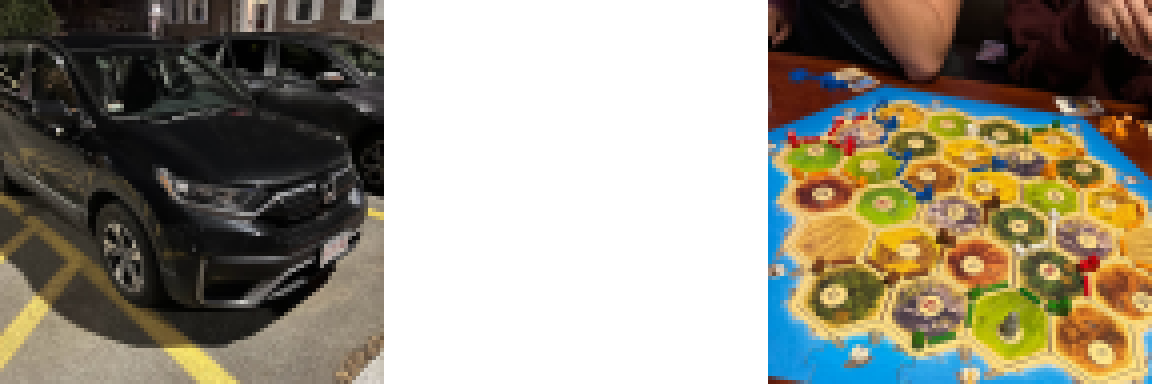
Consider the following two 224x224 images from the author’s camera roll - one of a car, one not. We will test our Arduino project by loading both of these images and executing the compiled model on them.

Currently, these are 224x224 PNG images we can download from Imgur. Before we can feed in these images, we’ll need to resize and convert them to raw data, which can be done with imagemagick.

It’s also challenging to load raw data onto an Arduino, as only C/CPP files (and similar) are compiled. We can work around this by embedding our raw data in a hard-coded C array with the built-in utility bin2c that will output a file like below:

static const unsigned char CAR_IMAGE[] = {
  0x22,0x23,0x14,0x22,
  ...
  0x07,0x0e,0x08,0x08
};

We can do both of these things with a few lines of Bash code:

mkdir -p ~/tests
curl "https://i.imgur.com/JBbEhxN.png" -o ~/tests/car_224.png
convert ~/tests/car_224.png -resize 64 ~/tests/car_64.png
stream ~/tests/car_64.png ~/tests/car.raw
bin2c -c -st ~/tests/car.raw --name CAR_IMAGE > ~/models/project/car.c

curl "https://i.imgur.com/wkh7Dx2.png" -o ~/tests/catan_224.png
convert ~/tests/catan_224.png -resize 64 ~/tests/catan_64.png
stream ~/tests/catan_64.png ~/tests/catan.raw
bin2c -c -st ~/tests/catan.raw --name CATAN_IMAGE > ~/models/project/catan.c

Writing our Arduino Script

We now need a little bit of Arduino code to read the two binary arrays we just generated, run the model on them, and log the output to the serial monitor. This file will replace arduino_sketch.ino as the main file of our sketch. You’ll have to copy this code in manually..

#include "src/model.h"
#include "car.c"
#include "catan.c"

void setup() {
  Serial.begin(9600);
  TVMInitialize();
}

void loop() {
  uint8_t result_data[2];
  Serial.println("Car results:");
  TVMExecute(const_cast<uint8_t*>(CAR_IMAGE), result_data);
  Serial.print(result_data[0]); Serial.print(", ");
  Serial.print(result_data[1]); Serial.println();

  Serial.println("Other object results:");
  TVMExecute(const_cast<uint8_t*>(CATAN_IMAGE), result_data);
  Serial.print(result_data[0]); Serial.print(", ");
  Serial.print(result_data[1]); Serial.println();

  delay(1000);
}

Compiling Our Code

Now that our project has been generated, TVM’s job is mostly done! We can still call arduino_project.build() and arduino_project.upload(), but these just use arduino-cli’s compile and flash commands underneath. We could also begin autotuning our model, but that’s a subject for a different tutorial. To finish up, we’ll verify no compiler errors are thrown by our project:

shutil.rmtree(f"{FOLDER}/models/project/build", ignore_errors=True)
arduino_project.build()
print("Compilation succeeded!")

Compilation succeeded!

Uploading to Our Device

The very last step is uploading our sketch to an Arduino to make sure our code works properly. Unfortunately, we can’t do that from Google Colab, so we’ll have to download our sketch. This is simple enough to do - we’ll just turn our project into a .zip archive, and call files.download. If you’re running on Google Colab, you’ll have to uncomment the last two lines to download the file after writing it.

ZIP_FOLDER = f"{FOLDER}/models/project"
shutil.make_archive(ZIP_FOLDER, "zip", ZIP_FOLDER)
# from google.colab import files
# files.download(f"{FOLDER}/models/project.zip")

From here, we’ll need to open it in the Arduino IDE. You’ll have to download the IDE as well as the SDK for whichever board you are using. For certain boards like the Sony SPRESENSE, you may have to change settings to control how much memory you want the board to use.

Expected Results

If all works as expected, you should see the following output on a Serial monitor:

Car results:
255, 0
Other object results:
0, 255

The first number represents the model’s confidence that the object is a car and ranges from 0-255. The second number represents the model’s confidence that the object is not a car and is also 0-255. These results mean the model is very sure that the first image is a car, and the second image is not (which is correct). Hence, our model is working!

Summary

In this tutorial, we used transfer learning to quickly train an image recognition model to identify cars. We modified its input dimensions and last few layers to make it better at this, and to make it faster and smaller. We then quantified the model and compiled it using TVM to create an Arduino sketch. Lastly, we tested the model using two static images to prove it works as intended.

Next Steps

From here, we could modify the model to read live images from the camera - we have another Arduino tutorial for how to do that on GitHub. Alternatively, we could also use TVM’s autotuning capabilities to dramatically improve the model’s performance.