2D Convolution Optimization

Author: Thierry Moreau

This tutorial provides an overview on how to use TVM to map a 2D convolution workload efficiently on the VTA design. We recommend covering the Matrix Multiply Blocking tutorial first.

2D convolution is dominant in most computer vision deep neural networks. In this tutorial, we will demonstrate TVM schedule optimizations to map 2D convolution operators in NCHW layout onto VTA. We also introduce the notion of latency hiding, which allows us to maximize VTA’s compute and memory resource utilization.

RPC Setup

We start by programming the Pynq’s FPGA and building its RPC runtime.

from __future__ import absolute_import, print_function

import os
import tvm
import tvm.testing
from tvm import te
import vta
import numpy as np

from tvm import rpc
from tvm.contrib import utils
from vta.testing import simulator

# Load VTA parameters from the 3rdparty/vta-hw/config/vta_config.json file
env = vta.get_env()

# We read the Pynq RPC host IP address and port number from the OS environment
host = os.environ.get("VTA_RPC_HOST", "192.168.2.99")
port = int(os.environ.get("VTA_RPC_PORT", "9091"))

# We configure both the bitstream and the runtime system on the Pynq
# to match the VTA configuration specified by the vta_config.json file.
if env.TARGET == "pynq":

    # Make sure that TVM was compiled with RPC=1
    assert tvm.runtime.enabled("rpc")
    remote = rpc.connect(host, port)

    # Reconfigure the JIT runtime
    vta.reconfig_runtime(remote)

    # Program the FPGA with a pre-compiled VTA bitstream.
    # You can program the FPGA with your own custom bitstream
    # by passing the path to the bitstream file instead of None.
    vta.program_fpga(remote, bitstream=None)

# In simulation mode, host the RPC server locally.
elif env.TARGET in ["sim", "tsim"]:
    remote = rpc.LocalSession()

Computation Declaration

As a first step, we need to describe our 2D convolution computation in NCHW format.

We define the 2D convolution shape by the batch size, spatial dimensions, input channels, output channels, kernel dimensions, kernel dimensions, padding dimensions, and stride dimensions.

We pick the shape of the 9th convolutional layer of the ResNet-18 architecture as our convolution workload parameters.

We’ve added extra operators to the 2D convolution that apply shifting and clipping to the output in order to mimic a fixed-point convolution followed by a rectified linear activation. We describe the TVM dataflow graph of the 2D convolution layer below:

This computation is intentionally too large to fit onto VTA’s on-chip buffers all at once. Therefore in the scheduling phase we’ll rely on computation blocking strategies to break the computation down into manageable chunks.

Note

Spatial padding

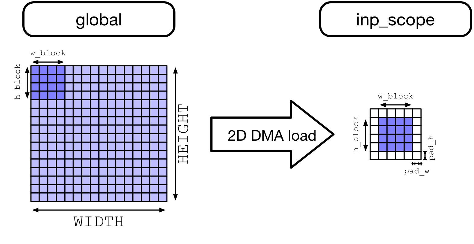
Note that we’ll need to import the TOPI library to apply spatial padding on the input feature map tensor. Spatial padding facilitates blocking in the context of 2D convolutions due to the fact that the same (x, y) spatial location of the input feature map of any given layer is read more than once if the convolution kernel window size is greater than one. On CPUs, and GPUs, one way to increase efficiency of memory accesses when parallelizing work is spatial packing, which requires data re-layout. VTA load DMA engine can insert padding automatically so that the original input feature map does not have to be re-packed in memory.

We show the effect of VTA’s on the fly spatial padding when data is being loaded from DRAM into VTA’s SRAM, following a 2D strided and padded memory read.

from tvm import topi

# 2D convolution layer dimensions taken from ResNet-18 architecture
# (9th convolutional layer)
batch_size = 1
height = 14
width = 14
in_channels = 256
out_channels = 256
kernel_h = 3
kernel_w = 3
pad_h = 1
pad_w = 1
stride_h = 1
stride_w = 1
assert batch_size % env.BATCH == 0
assert in_channels % env.BLOCK_IN == 0
assert out_channels % env.BLOCK_OUT == 0

# Input feature map: (N, IC, H, W, n, ic)
data_shape = (
    batch_size // env.BATCH,
    in_channels // env.BLOCK_IN,
    height,
    width,
    env.BATCH,
    env.BLOCK_IN,
)
# Kernel: (OC, IC, H, W, oc, ic)
kernel_shape = (
    out_channels // env.BLOCK_OUT,
    in_channels // env.BLOCK_IN,
    kernel_h,
    kernel_w,
    env.BLOCK_OUT,
    env.BLOCK_IN,
)
# Derive output feature map dimensions
fout_height = (height + 2 * pad_h - kernel_h) // stride_h + 1
fout_width = (width + 2 * pad_w - kernel_w) // stride_w + 1
# Output feature map: (N, OC, H, W, n, oc)
output_shape = (
    batch_size // env.BATCH,
    out_channels // env.BLOCK_OUT,
    fout_height,
    fout_width,
    env.BATCH,
    env.BLOCK_OUT,
)

# Convolution reduction axes
dy = te.reduce_axis((0, kernel_h), name="dy")
dx = te.reduce_axis((0, kernel_w), name="dx")
ic = te.reduce_axis((0, in_channels // env.BLOCK_IN), name="ic")
ic_tns = te.reduce_axis((0, env.BLOCK_IN), name="ic_tns")

# Input placeholder tensors
data = te.placeholder(data_shape, name="data", dtype=env.inp_dtype)
kernel = te.placeholder(kernel_shape, name="kernel", dtype=env.wgt_dtype)

# Copy buffers:
#   Apply spatial padding to input feature map
data_buf = topi.nn.pad(data, [0, 0, pad_h, pad_w, 0, 0], name="data_buf")
kernel_buf = te.compute(kernel_shape, lambda *i: kernel(*i), "kernel_buf")

# Declare 2D convolution
res_conv = te.compute(
    output_shape,
    lambda bo, co, i, j, bi, ci: te.sum(
        data_buf[bo, ic, i * stride_h + dy, j * stride_w + dx, bi, ic_tns].astype(env.acc_dtype)
        * kernel_buf[co, ic, dy, dx, ci, ic_tns].astype(env.acc_dtype),
        axis=[ic, dy, dx, ic_tns],
    ),
    name="res_conv",
)

# Add shift stage for fix-point normalization
res_shr = te.compute(output_shape, lambda *i: res_conv(*i) >> 8, name="res_shr")

# Apply clipping between (0, input max value)
inp_max = (1 << (env.INP_WIDTH - 1)) - 1
res_max = te.compute(output_shape, lambda *i: tvm.te.max(res_shr(*i), 0), "res_max")
res_min = te.compute(output_shape, lambda *i: tvm.te.min(res_max(*i), inp_max), "res_min")

# Result Tensor
res = te.compute(output_shape, lambda *i: res_min(*i).astype(env.inp_dtype), name="res")

Scheduling the Computation

We’ll look at a set of schedule transformations necessary to map the 2D convolution onto VTA in an efficient fashion. Those include:

• Computation blocking

• Virtual threading to increase compute utilization

• Lowering to VTA hardware intrinsics

# Create TVM schedule
s = te.create_schedule(res.op)
# Let's look at the default TVM schedule
print(tvm.lower(s, [data, kernel, res], simple_mode=True))

Blocking the Computation

The 2D convolution is by default too large for activations or kernel weights to fit on VTA’s on-chip buffers all at once. We apply blocking along input channels, output channels, and along the height spatial dimensions. We don’t apply blocking along the width spatial dimension since it’s the innermost dimension in the NCHW layout (and consequently to increase locality, it’s best not to block along the innermost dimension).

# Let's define tiling sizes
b_block = 1 // env.BATCH
oc_block = 128 // env.BLOCK_OUT
ic_block = 16 // env.BLOCK_IN
h_block = 7
w_block = 14

# Tile the output tensor along the spatial and output channel dimensions
# (since by default we are doing single batch inference, the split along
#  the batch dimension has no effect)
b, oc, y, x, b_tns, oc_tns = s[res].op.axis
b_out, b_inn = s[res].split(b, factor=b_block)
oc_out, oc_inn = s[res].split(oc, factor=oc_block)
y_out, y_inn = s[res].split(y, factor=h_block)
x_out, x_inn = s[res].split(x, factor=w_block)
s[res].reorder(b_out, oc_out, y_out, x_out, b_inn, oc_inn, y_inn, x_inn, b_tns, oc_tns)

# Move intermediate computation into each output compute tile
s[res_conv].compute_at(s[res], x_out)
s[res_shr].compute_at(s[res], x_out)
s[res_max].compute_at(s[res], x_out)
s[res_min].compute_at(s[res], x_out)

# Apply additional loop split along reduction axis (input channel)
b_inn, oc_inn, y_inn, x_inn, b_tns, oc_tns = s[res_conv].op.axis
ic_out, ic_inn = s[res_conv].split(ic, factor=ic_block)

# Reorder axes.
# 1) Group the VTA tensor axes in the inner most position: b_tns, oc_tns, ic_tns
#    to allow TVM to tensorize.
# 2) We move the ic_out axis all the way out of the convolution loop to block
#    along the reduction axis.
# 3) Now we re-order the block axes: b_inn, oc_inn, y_inn, x_inn, ic_inn, dy, dx.
#    VTA runtime/hardware requires us to write to a different output feature map
#    location for every VTA tensor operation.
#    This restriction requires us to order one of oc_inn, y_inn or x_inn right
#    before b_tns, since they all affect output feature map indexing.
#    Therefore, we choose to bring x_inn inside as shown below.
s[res_conv].reorder(ic_out, b_inn, oc_inn, y_inn, ic_inn, dy, dx, x_inn, b_tns, oc_tns, ic_tns)

Virtual Threading

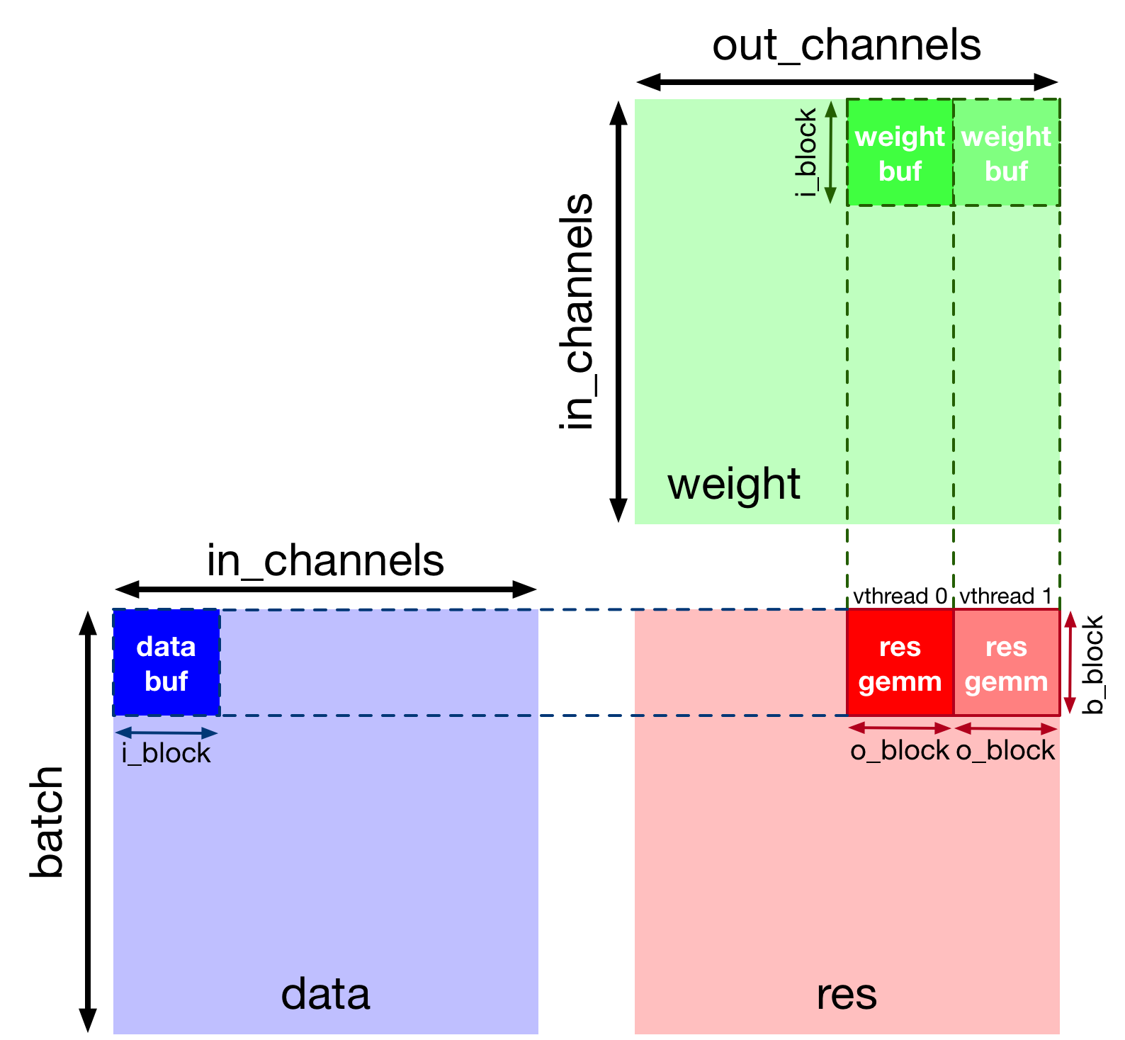
Virtual threading is a mechanism that increases task-level pipeline parallelism in the VTA hardware design. Put it another way, it increases compute resource utilization by hiding memory access latency.

In the implementation below, virtual threading distributes work across two threads split along the output channel axis. We show how work is split when computing the 2D convolution in the figure below.

# VTA only supports 2 virtual threads
v_threads = 2

# Perform virtual thread split along output channel outer axis
_, tx = s[res].split(oc_out, factor=v_threads)
s[res].reorder(tx, b_out)
s[res].bind(tx, te.thread_axis("cthread"))

# Let's look at the current TVM schedule after blocking and virtual threading
print(tvm.lower(s, [data, kernel, res], simple_mode=True))

Lowering Copies to DMA Transfers

Next we set the buffer scopes to the corresponding on-chip VTA SRAM buffers. We move the load loops into the 2D convolution computation loop to stage memory loads such that they fit in the on-chip SRAM buffers. Finally we annotate the load/store loop outer axes with the DMA copy pragma to perform bulk memory transfers on VTA.

# Set scope of SRAM buffers
s[data_buf].set_scope(env.inp_scope)
s[kernel_buf].set_scope(env.wgt_scope)
s[res_conv].set_scope(env.acc_scope)
s[res_shr].set_scope(env.acc_scope)
s[res_min].set_scope(env.acc_scope)
s[res_max].set_scope(env.acc_scope)

# Block data and kernel cache reads
s[data_buf].compute_at(s[res_conv], ic_out)
s[kernel_buf].compute_at(s[res_conv], ic_out)

# Use DMA copy pragma on DRAM->SRAM operations
s[data_buf].pragma(s[data_buf].op.axis[0], env.dma_copy)
s[kernel_buf].pragma(s[kernel_buf].op.axis[0], env.dma_copy)

# Use DMA copy pragma on SRAM->DRAM operation in each result block
# (this implies that these copies should be performed along b_inn,
# or result axis 4)
s[res].pragma(s[res].op.axis[4], env.dma_copy)

Lowering Computation to VTA Compute Intrinsics

The last phase is to lower the computation loops down to VTA hardware intrinsics by mapping the 2D convolution to tensor intrinsics, and mapping the shift, and clipping computation to the vector ALU.

# Apply tensorization over the batch tensor tile axis
s[res_conv].tensorize(b_tns, env.gemm)

# Add an ALU pragma over the shift and clipping operations
s[res_shr].pragma(s[res_shr].op.axis[0], env.alu)
s[res_min].pragma(s[res_min].op.axis[0], env.alu)
s[res_max].pragma(s[res_max].op.axis[0], env.alu)

# Let's look at the final lowered TVM schedule after lowering memory
# loads/stores down to DMA copy intrinsics, and the computation down to
# VTA compute intrinsics.
print(vta.lower(s, [data, kernel, res], simple_mode=True))

TVM Compilation and Verification

After specifying the schedule, we can compile it into a TVM function. We save the module so we can send it over RPC. We run the function and verify it against a numpy implementation to ensure correctness.

# This library facilitates 2D convolution testing
from tvm.topi.testing import conv2d_nchw_python

# Compile the TVM module
with vta.build_config(disabled_pass={"tir.CommonSubexprElimTIR"}):
    my_conv = vta.build(
        s, [data, kernel, res], tvm.target.Target("ext_dev", host=env.target_host), name="my_conv"
    )
temp = utils.tempdir()
my_conv.save(temp.relpath("conv2d.o"))
remote.upload(temp.relpath("conv2d.o"))
f = remote.load_module("conv2d.o")

# Get the remote device context
ctx = remote.ext_dev(0)

# Initialize the data and kernel arrays randomly in the int range
# of (-128, 128] in NCHW layout
data_np = np.random.randint(-128, 128, size=(batch_size, in_channels, height, width)).astype(
    data.dtype
)
kernel_np = np.random.randint(
    -128, 128, size=(out_channels, in_channels, kernel_h, kernel_w)
).astype(kernel.dtype)

# Apply packing to the data and kernel arrays from a 2D NCHW
# to a 4D NCHWnc packed layout
data_packed = data_np.reshape(
    batch_size // env.BATCH, env.BATCH, in_channels // env.BLOCK_IN, env.BLOCK_IN, height, width
).transpose((0, 2, 4, 5, 1, 3))

kernel_packed = kernel_np.reshape(
    out_channels // env.BLOCK_OUT,
    env.BLOCK_OUT,
    in_channels // env.BLOCK_IN,
    env.BLOCK_IN,
    kernel_h,
    kernel_w,
).transpose((0, 2, 4, 5, 1, 3))

# Format the input/output arrays with tvm.nd.array to the DLPack standard
data_nd = tvm.nd.array(data_packed, ctx)
kernel_nd = tvm.nd.array(kernel_packed, ctx)
res_nd = tvm.nd.array(np.zeros(output_shape).astype(res.dtype), ctx)

# Clear stats
if env.TARGET in ["sim", "tsim"]:
    simulator.clear_stats()

# Invoke the module to perform the computation
f(data_nd, kernel_nd, res_nd)

# Verify against numpy implementation
res_ref = conv2d_nchw_python(
    data_np.astype(env.acc_dtype),
    kernel_np.astype(env.acc_dtype),
    (stride_h, stride_w),
    (pad_h, pad_w),
).astype(env.acc_dtype)
res_ref = res_ref >> env.INP_WIDTH
res_ref = np.clip(res_ref, 0, inp_max)
res_ref = res_ref.astype(res.dtype)
res_ref = res_ref.reshape(
    (
        batch_size // env.BATCH,
        env.BATCH,
        out_channels // env.BLOCK_OUT,
        env.BLOCK_OUT,
        fout_height,
        fout_width,
    )
).transpose((0, 2, 4, 5, 1, 3))
tvm.testing.assert_allclose(res_ref, res_nd.numpy())

# Print stats
if env.TARGET in ["sim", "tsim"]:
    sim_stats = simulator.stats()
    print("Execution statistics:")
    for k, v in sim_stats.items():
        print("\t{:<16}: {:>16}".format(k, v))

print("Successful 2D convolution test!")

Summary

This tutorial demonstrates how TVM scheduling primitives can be used to lower 2D convolution onto hardware accelerator intrinsics, making use of hardware specific optimizations, such as latency hiding with virtual threading.